Fourier analysis

Fourier transforms
Continuous Fourier transform
Fourier series
Discrete Fourier transform
Discrete-time Fourier transform
Related transforms

In mathematics, Fourier analysis is a subject area which grew from the study of Fourier series. The subject began with the study of the way general functions may be represented by sums of simpler trigonometric functions. Fourier analysis is named after Joseph Fourier, who showed that representing a function by a trigonometric series greatly simplifies the study of heat propagation.

Today, the subject of Fourier analysis encompasses a vast spectrum of mathematics. In the sciences and engineering, the process of decomposing a function into simpler pieces is often called Fourier analysis, while the operation of rebuilding the function from these pieces is known as Fourier synthesis. In mathematics, the term Fourier analysis often refers to the study of both operations.

The decomposition process itself is called a Fourier transform. The transform is often given a more specific name which depends upon the domain and other properties of the function being transformed. Moreover, the original concept of Fourier analysis has been extended over time to apply to more and more abstract and general situations, and the general field is often known as harmonic analysis. Each transform used for analysis (see list of Fourier-related transforms) has a corresponding inverse transform that can be used for synthesis.

1 Applications
- 1.1 Applications in signal processing
2 Variants of Fourier analysis
3 History
4 Interpretation in terms of time and frequency
5 See also
6 Notes
7 References
8 External links

Applications

Fourier analysis has many scientific applications — in physics, partial differential equations, number theory, combinatorics, signal processing, imaging, probability theory, statistics, option pricing, cryptography, numerical analysis, acoustics, oceanography, optics, diffraction, geometry, and other areas.

This wide applicability stems from many useful properties of the transforms:

The transforms are linear operators and, with proper normalization, are unitary as well (a property known as Parseval's theorem or, more generally, as the Plancherel theorem, and most generally via Pontryagin duality)(Rudin 1990).
The transforms are usually invertible, and when they are, the inverse transform has a similar form to the forward transform.
The exponential functions are eigenfunctions of differentiation, which means that this representation transforms linear differential equations with constant coefficients into ordinary algebraic ones (Evans 1998). (For example, in a linear time-invariant physical system, frequency is a conserved quantity, so the behavior at each frequency can be solved independently.)
By the convolution theorem, Fourier transforms turn the complicated convolution operation into simple multiplication, which means that they provide an efficient way to compute convolution-based operations such as polynomial multiplication and multiplying large numbers (Knuth 1997).
The discrete version of the Fourier transform (see below) can be evaluated quickly on computers using fast Fourier transform (FFT) algorithms. (Conte & de Boor 1980)

Fourier transformation is also useful as a compact representation of a signal. For example, JPEG compression uses a variant of the Fourier transformation (discrete cosine transform) of small square pieces of a digital image. The Fourier components of each square are rounded to lower arithmetic precision, and weak components are eliminated entirely, so that the remaining components can be stored very compactly. In image reconstruction, each Fourier-transformed image square is reassembled from the preserved approximate components, and then inverse-transformed to produce an approximation of the original image.

Applications in signal processing

When processing signals, such as audio, radio waves, light waves, seismic waves, and even images, Fourier analysis can isolate individual components of a compound waveform, concentrating them for easier detection and/or removal. A large family of signal processing techniques consist of Fourier-transforming a signal, manipulating the Fourier-transformed data in a simple way, and reversing the transformation.

Some examples include:

Telephone dialing; the touch-tone signals for each telephone key, when pressed, are each a sum of two separate tones (frequencies). Fourier analysis can be used to separate (or analyze) the telephone signal, to reveal the two component tones and therefore which button was pressed.
Removal of unwanted frequencies from an audio recording (used to eliminate hum from leakage of AC power into the signal, to eliminate the stereo subcarrier from FM radio recordings);
Noise gating of audio recordings to remove quiet background noise by eliminating Fourier components that do not exceed a preset amplitude;
Equalization of audio recordings with a series of bandpass filters;
Digital radio reception with no superheterodyne circuit, as in a modern cell phone or radio scanner;
Image processing to remove periodic or anisotropic artifacts such as jaggies from interlaced video, stripe artifacts from strip aerial photography, or wave patterns from radio frequency interference in a digital camera;
Cross correlation of similar images for co-alignment;
X-ray crystallography to reconstruct a crystal structure from its diffraction pattern;
Fourier transform ion cyclotron resonance mass spectrometry to determine the mass of ions from the frequency of cyclotron motion in a magnetic field.
Many other forms of spectroscopy also rely upon Fourier Transforms to determine the three-dimensional structure and/or identity of the sample being analyzed, including Infrared and Nuclear Magnetic Resonance spectroscopies.
Generation of sound spectrograms used to analyze sounds.

Variants of Fourier analysis

Fourier analysis has different forms, some of which have different names. The more common variants are shown below. The different names usually reflect different properties of the function or data being analyzed. The resultant transforms can be seen as special cases or generalizations of each other.

(Continuous) Fourier transform

Main article: Fourier Transform

Most often, the unqualified term Fourier transform refers to the transform of functions of a continuous real argument, such as time (t). In this case the Fourier transform describes a function ƒ(t) in terms of basic complex exponentials of various frequencies. In terms of ordinary frequency ν, the Fourier transform is given by the complex number:

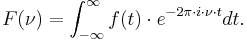
$F(\nu) = \int_{-\infty}^{\infty} f(t) \cdot e^{- 2\pi \cdot i \cdot \nu \cdot t} dt.$

Evaluating this quantity for all values of ν produces the frequency-domain function.

See Fourier transform for even more information, including:

the inverse transform, F(ν) → ƒ(t)
conventions for amplitude normalization and frequency scaling/units
transform properties
tabulated transforms of specific functions
an extension/generalization for functions of multiple dimensions, such as images

Fourier series

Main article: Fourier series

Fourier analysis for functions defined on a circle, or equivalently for periodic functions, mainly focuses on the study of Fourier series. Suppose that ƒ(x) is a periodic function with period 2π, in this case one can attempt to decompose ƒ(x) as a sum of complex exponentials functions. The coefficients F(n) of the complex exponential in the sum are referred to as the Fourier coefficients for ƒ and are analogous to the "Fourier transform" of a function on the line (Katznelson 1976). The term Fourier series expansion or simply Fourier series refers to the infinite series that appears in the inverse transform. The Fourier coefficients of ƒ(x) are given by:

$F(n) = \frac{1}{2\pi} \int_{0}^{2\pi} f(x) e^{-i n x} \, dx,$

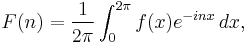
for all integers n. And the Fourier series of ƒ(x) is given by:

$f(x)=\sum_{n=-\infty}^\infty F(n) e^{i n x}.$

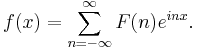
Equality may not always hold in the equation above and the study of the convergence of Fourier series is a central part of Fourier analysis of the circle.

Analysis of periodic functions or functions with limited duration

When ƒ(x) has finite duration (or compact support), a discrete subset of the values of its continuous Fourier transform is sufficient to reconstruct/represent the function ƒ(x) on its support. One such discrete set is obtained by treating the duration of the segment as if it is the period of a periodic function and computing the Fourier coefficients. Putting convergence issues aside, the Fourier series expansion will be a periodic function not the finite-duration function ƒ(x); but one period of the expansion will give the values of ƒ(x) on its support.

See Fourier series for more information, including:

Fourier series expansions for general periods,
transform properties,
historical development,
special cases and generalizations.

Discrete-time Fourier transform (DTFT)

For functions of an integer index, the discrete-time Fourier transform (DTFT) provides a useful frequency-domain transform.

A useful "discrete-time" function can be obtained by sampling a "continuous-time" function, s(t), which produces a sequence, s(nT), for integer values of n and some time-interval T. If information is lost, then only an approximation to the original transform, S(f), can be obtained by looking at one period of the periodic function:

$S_T(f) = \sum_{k=-\infty}^{\infty} S\left(f - \frac{k}{T}\right) \equiv \sum_{n=-\infty}^{\infty} \underbrace{T\cdot s(nT)}_{s[n]} \cdot e^{-i 2\pi f n T},$

which is the DTFT. The identity above is a result of the Poisson summation formula. The DTFT is also equivalent to the Fourier transform of a "continuous" function that is constructed by using the s[n] sequence to modulate a Dirac comb.

Applications of the DTFT are not limited to sampled functions. It can be applied to any discrete sequence. See Discrete-time Fourier transform for more information on this and other topics, including:

the inverse transform
normalized frequency units
windowing (finite-length sequences)
transform properties
tabulated transforms of specific functions

Discrete Fourier transform (DFT)

Main article: Discrete Fourier transform

Since the DTFT is also a continuous Fourier transform (of a comb function), the Fourier series also applies to it. Thus, when s[n] is periodic, with period N, S_T(ƒ) is another Dirac comb function, modulated by the coefficients of a Fourier series. And the integral formula for the coefficients simplifies to:

$S[k] = \sum_{n=0}^{N-1} s[n] \cdot e^{-i 2 \pi \frac{k}{N} n}$ for all integer values of k.

Since the DTFT is periodic, so is S[k]. And it has the same period (N) as the input function. This transform is also called DFT, particularly when only one period of the output sequence is computed from one period of the input sequence.

When s[n] is not periodic, but its non-zero portion has finite duration (N), S_T(ƒ) is continuous and finite-valued. But a discrete subset of its values is sufficient to reconstruct/represent the (finite) portion of s[n] that was analyzed. The same discrete set is obtained by treating N as if it is the period of a periodic function and computing the Fourier series coefficients / DFT.

The inverse transform of S[k] does not produce the finite-length sequence, s[n], when evaluated for all values of n. (It takes the inverse of S_T(ƒ) to do that.) The inverse DFT can only reproduce the entire time-domain if the input happens to be periodic (forever). Therefore it is often said that the DFT is a transform for Fourier analysis of finite-domain, discrete-time functions. An alternative viewpoint is that the periodicity is the time-domain consequence of approximating the continuous-domain function, S_T(ƒ), with the discrete subset, S[k]. N can be larger than the actual non-zero portion of s[n]. The larger it is, the better the approximation (also known as zero-padding).

The DFT can be computed using a fast Fourier transform (FFT) algorithm, which makes it a practical and important transformation on computers.

See Discrete Fourier transform for much more information, including:

the inverse transform
transform properties
applications
tabulated transforms of specific functions

Fourier transforms summary

The following table recaps the four basic forms discussed above, highlighting the duality of the properties of discreteness and periodicity. I.e., if the signal representation in one domain has either (or both) of those properties, then its transform representation to the other domain has the other property (or both).

Name	Time domain		Frequency domain		Function's
Name	Domain property	Function property	Domain property	Function property	Energy	Average power
(Continuous) Fourier transform (FT)	Continuous	Aperiodic	Continuous	Aperiodic	Finite	Infinitesimal
Discrete-time Fourier transform (DTFT)	Discrete	Aperiodic	Continuous	Periodic (ƒ_s)	Finite	Infinitesimal
Fourier series (FS)	Continuous	Periodic ( $\tau$ )	Discrete	Aperiodic	Infinite	Finite
Discrete Fourier series^[1] (DFS)	Discrete	Periodic (N)^[2]	Discrete	Periodic (N)	Infinite	Finite

Fourier transforms on arbitrary locally compact abelian topological groups

The Fourier variants can also be generalized to Fourier transforms on arbitrary locally compact abelian topological groups, which are studied in harmonic analysis; there, the Fourier transform takes functions on a group to functions on the dual group. This treatment also allows a general formulation of the convolution theorem, which relates Fourier transforms and convolutions. See also the Pontryagin duality for the generalized underpinnings of the Fourier transform.

Time–frequency transforms

In signal processing terms, a function (of time) is a representation of a signal with perfect time resolution, but no frequency information, while the Fourier transform has perfect frequency resolution, but no time information.

As alternatives to the Fourier transform, in time–frequency analysis, one uses time–frequency transforms to represent signals in a form that has some time information and some frequency information – by the uncertainty principle, there is a trade-off between these. These can be generalizations of the Fourier transform, such as the short-time Fourier transform or fractional Fourier transform, or can use different functions to represent signals, as in wavelet transforms and chirplet transforms, with the wavelet analog of the (continuous) Fourier transform being the continuous wavelet transform.

History

A primitive form of harmonic series dates back to ancient Babylonian mathematics, where they were used to compute ephemerides (tables of astronomical positions).^[3]

In modern times, variants of the discrete Fourier transform were used by Alexis Clairaut in 1754 to compute an orbit,^[4] which has been described as the first formula for the DFT,^[5] and in 1759 by Joseph Louis Lagrange, in computing the coefficients of a trigonometric series for a vibrating string.^[6] Technically, Clairaut's work was a cosine-only series (a form of discrete cosine transform), while Lagrange's work was a sine-only series (a form of discrete sine transform); a true cosine+sine DFT was used by Gauss in 1805 for trigonometric interpolation of asteroid orbits.^[7] Euler and Lagrange both discretized the vibrating string problem, using what would today be called samples.^[6]

An early modern development toward Fourier analysis was the 1770 paper Réflexions sur la résolution algébrique des équations by Lagrange, which in the method of Lagrange resolvents used a complex Fourier decomposition to study the solution of a cubic:^[8] Lagrange transformed the roots $x_1,x_2,x_3$ into the resolvents:

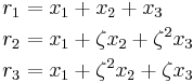
$\begin{align} r_1 &= x_1 + x_2 + x_3\\ r_2 &= x_1 + \zeta x_2 + \zeta^2 x_3\\ r_3 &= x_1 + \zeta^2 x_2 + \zeta x_3 \end{align}$

where ζ is a cubic root of unity, which is the DFT of order 3.

A number of authors, notably Jean le Rond d'Alembert, , and Carl Friedrich Gauss used trigonometric series to study the heat equation, but the breakthrough development was the 1807 paper Mémoire sur la propagation de la chaleur dans les corps solides by Joseph Fourier, whose crucial insight was to model all functions by trigonometric series, introducing the Fourier series.

Historians are divided as to how much to credit Lagrange and others for the development of Fourier theory: Daniel Bernoulli and Leonhard Euler had introduced trigonometric representations of functions,^[5] and Lagrange had given the Fourier series solution to the wave equation,^[5] so Fourier's contribution was mainly the bold claim that an arbitrary function could be represented by a Fourier series.^[5]

The subsequent development of the field is known as harmonic analysis, and is also an early instance of representation theory.

The first fast Fourier transform (FFT) algorithm for the DFT was discovered around 1805 by Carl Friedrich Gauss when interpolating measurements of the orbit of the asteroids Juno and Pallas, although that particular FFT algorithm is more often attributed to its modern rediscoverers Cooley and Tukey.^[7]^[9]

Interpretation in terms of time and frequency

In signal processing, the Fourier transform often takes a time series or a function of continuous time, and maps it into a frequency spectrum. That is, it takes a function from the time domain into the frequency domain; it is a decomposition of a function into sinusoids of different frequencies; in the case of a Fourier series or discrete Fourier transform, the sinusoids are harmonics of the fundamental frequency of the function being analyzed.

When the function ƒ is a function of time and represents a physical signal, the transform has a standard interpretation as the frequency spectrum of the signal. The magnitude of the resulting complex-valued function F at frequency ω represents the amplitude of a frequency component whose initial phase is given by the phase of F.

Fourier transforms are not limited to functions of time, and temporal frequencies. They can equally be applied to analyze spatial frequencies, and indeed for nearly any function domain. This justifies their use in branches such diverse as image processing, heat conduction and automatic control.

Notes

↑ The discrete Fourier series (DFS) are practically the same as the discrete Fourier transform (DFT).
↑ Or N is simply the length of a finite sequence. In either case, the inverse DFT formula produces a periodic function, s[n].
↑ Prestini, Elena (2004), The evolution of applied harmonic analysis: models of the real world, Birkhäuser, ISBN 978 0 81764125 2, http://books.google.com/?id=fye--TBu4T0C , p. 62
Rota, Gian-Carlo; Palombi, Fabrizio (1997), Indiscrete thoughts, Birkhäuser, ISBN 978 0 81763866 5, http://books.google.com/?id=H5smrEExNFUC , p. 11
Neugebauer, Otto (1969) [1957], The Exact Sciences in Antiquity (2 ed.), Dover Publications, ISBN 978-048622332-2, http://books.google.com/?id=JVhTtVA2zr8C
Brack-Bernsen, Lis; Brack, Matthias, Analyzing shell structure from Babylonian and modern times, http://arxiv.org/abs/physics/0310126
↑ Terras, Audrey (1999), Fourier analysis on finite groups and applications, Cambridge University Press, ISBN 978 0 52145718 7, http://books.google.com/?id=-B2TA669dJMC , p. 30
↑ ^5.0 ^5.1 ^5.2 ^5.3 Briggs, William L.; Henson, Van Emden (1995), The DFT : an owner's manual for the discrete Fourier transform, SIAM, ISBN 978 0 89871342 8, http://books.google.com/?id=coq49_LRURUC , p. 4
↑ ^6.0 ^6.1 Briggs, William L.; Henson, Van Emden (1995), The DFT: an owner's manual for the discrete Fourier transform, SIAM, ISBN 978 0 89871342 8, http://books.google.com/?id=coq49_LRURUC , p. 2
↑ ^7.0 ^7.1 Heideman, M. T., D. H. Johnson, and C. S. Burrus, "Gauss and the history of the fast Fourier transform," IEEE ASSP Magazine, 1, (4), 14–21 (1984)
↑ Knapp, Anthony W. (2006), Basic algebra, Springer, ISBN 978 0 81763248 9, http://books.google.com/?id=KVeXG163BggC , p. 501
↑ Terras, Audrey (1999), Fourier analysis on finite groups and applications, Cambridge University Press, ISBN 978 0 52145718 7, http://books.google.com/?id=-B2TA669dJMC , p. 31

References

Conte, S. D.; de Boor, Carl (1980), Elementary Numerical Analysis (Third ed.), New York: McGraw Hill, Inc., ISBN 0-07-012447-7, ISBN 0070662282
Evans, L. (1998), Partial Differential Equations, American Mathematical Society, ISBN 3540761241
Kamen, E.W., and B.S. Heck. "Fundamentals of Signals and Systems Using the Web and Matlab". ISBN 0-13-017293-6
Knuth, Donald E. (1997), The Art of Computer Programming Volume 2: Seminumerical Algorithms (3rd ed.), Section 4.3.3.C: Discrete Fourier transforms, pg.305: Addison-Wesley Professional, ISBN 0201896842
Polyanin, A.D., and A.V. Manzhirov (1998). Handbook of Integral Equations, CRC Press, Boca Raton. ISBN 0-8493-2876-4
Rudin, Walter (1990), Fourier Analysis on Groups, Wiley-Interscience, ISBN 047152364X
Smith, Steven W. (1999), The Scientist and Engineer's Guide to Digital Signal Processing (Second ed.), San Diego, Calif.: California Technical Publishing, ISBN 0-9660176-3-3, http://www.dspguide.com/pdfbook.htm
Stein, E.M., and G. Weiss (1971). Introduction to Fourier Analysis on Euclidean Spaces. Princeton University Press. ISBN 0-691-08078-X

External links

Tables of Integral Transforms at EqWorld: The World of Mathematical Equations.
An Intuitive Explanation of Fourier Theory by Steven Lehar.
Lectures on Image Processing: A collection of 18 lectures in pdf format from Vanderbilt University. Lecture 6 is on the 1- and 2-D Fourier Transform. Lectures 7-15 make use of it., by Alan Peters